Texture mapping, part 3
Hi, this is the third and final installment of my three-part series on texture mapping. After the first part (by Boreal) covered affine texture mapping (which is basically a 2D technique applied to 3D, and as such often distorts textures in spectacular ways), and the second part (by me) covered perspective-correct texture mapping, this article will cover approximated techniques which results in better results than affine texturing and better speed than perspective-correct mapping; I'll also cover briefly mipmapping.
The five techniques that I'll analyze are constant-Z mapping, linear approximation, scanline subdivision, parabolic approximation, and Bresenham (aka hyperbolic texture mapping).
Before starting, let me remind you of the conventions I'm using: X and Y are screen coordinates, u and v are texture coordinates, xyz are 3-D coordinates; finally m and n are two "magic coordinates", linear in screen space, such that u=m/(1/z) and v=n/(1/z).
Constant-Z mapping
Constant-Z is based on a very interesting remark. Since, as we saw, 1/z values are linear in screen-space with the following formula
1/z = -a/d X - b/d Y - c/d
lines with a slope of -a/b have a constant z: substitute
Y = -a/b X + Y0
and you have
1/z = -a/d X + a/d X - c/d + Y0 = Y0 - c/d
Hence, along these lines, u and v vary linearly in screen-space with these delta values:
         du = dm / (1/z)
         dv = dn / (1/z)
The basic algorithm then looks like this:
         for each constant-Z line in the polygon
             compute u, v, dm, dn as in part 2
             du = dm / (1/z)
             dv = dn / (1/z)
             for each point on Y = -a/b (X - X0) + Y0
                ... plot the (u,v) texel at (X,Y)...
                u = u + du
                v = v + dv
There are many problems though with this simple approach. The most evident is that you should take care of avoiding holes in the lines. There is an easy way to do this: use a Bresenham line scanner, (like the one that elmm/[KCN] explained in Hugi 24) and set the initial error as if you always scanned the lines from X=0 (if the line is scanned horizontally, that is if |a/b|<1) or from Y=0 if the line is scanned vertically, that is if |a/b|>1). The result is that each scanline is exactly the same as the previous one, only translated vertically.
So the inner loop becomes
        if |a/b|<1
            error = X0 * |a| % |b|
            for each X on the scanline
                ... plot the (u,v) texel at (X,Y)...
                error = error + |a|
                u = u + du
                v = v + dv
                if error >= |b| then
                    error = error - |b|
                    Y = Y + sgn(a/b)        // - if Y's grow upwards
        else
            error = X0 * |b| % |a|
            for each Y on the scanline
                ... plot the (u,v) texel at (X,Y)...
                error = error + |b|
                u = u + du
                v = v + dv
                if error >= |b| then
                    error = error - |a|
                    X = X + sgn(a/b)        // - if Y's grow upwards
Two other problems are less evident. Just look at these examples of how (intuitively) lines should be scanned
            1111                 45
           12222333             34567
          223333444455         23456789
         333444455            123456789ab
        444455               123456789abcde
       455                  0123456
The problem with the first example is that there are holes in the line labeled 5. This is most easily solved in the Bresenham inner loop, by checking if the X is in range and not plotting the pixel if so.
The problem with both examples is that I did not specify how to iterate through all constant-z lines. In the first example a reasonable choice seems to be to pick the leftmost pixel of each line and scan to the right; in the second example it seems to be to pick the bottom pixel and scan upwards. There are of course two symmetrical cases in which you should pick the rightmost point and scan to the left, or pick the topmost point and scan to the right. This complicates things a lot in the implementation of this algorithm.
And the result is not that good anyway, because the lines are not exactly constant-z. Since each of the two screen coordinates might be off by up to half a pixel with respect to the ideal constant-z line, the value of 1/z might be off by up to a/2d or b/2d. So, despite its promises, the algorithm is not correct for lines that are not horizontal, vertical or 45-degrees.
So, my position is: stay away from constant-Z.
Approximating perspective-correct texture mapping
Since mathematical tricks did not result in a good algorithm, let's assume that the only way to do really correct texture mapping is to loop on horizontal scanlines and do two divides per pixel. To save them, we should simply draw an approximation, though not one as brutal as affine texture mapping.
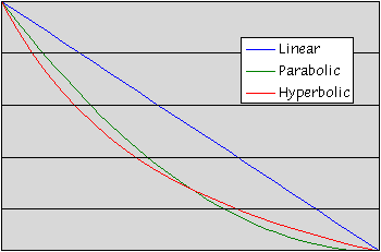
The four approximations that I will present are: a segment, many segments, a parabola, and a Bresenham-scanned hyperbola.
The graph below shows the linear approximation, the parabolic approximation, and the original hyperbola.
Two kind of linear approximations
This is quite a brutal way of approximating the hyperbola, as can be seen >from the graph.
This simply involves calculating the texture coordinates at both ends of each scan line and linearly interpolating them in between. This works well when there is a small angle between the view direction and the normal of the object being rendered, because in these cases the scanlines closely approximate constant-Z lines. However, as the angle increases the object starts to look distorted.
Just compute the u and v values at the two endpoints and interpolate in between:
    for each polygon
        compute A, B, C, D, E, F as in part 2
        scan convert it
        for each scanline Y
            X1 = leftmost point to be plotted (inclusive)
            X2 = rightmost point to be plotted (inclusive)

            // compute 1/z and 3D x, y at the endpoints
            zInv1 = -a/d * X1 - b/d * Y - c/d
            zInv2 = -a/d * X2 - b/d * Y - c/d
            x1 = X1 / zInv1
            x2 = X2 / zInv2
            y1 = Y1 / zInv1
            y2 = Y2 / zInv2

            // compute u, v at the endpoints and the interpolation step
            u1 = A * x1 + B * y1 + C
            v1 = D * x1 + E * y1 + F
            u2 = A * x2 + B * y2 + C
            v2 = D * x2 + E * y2 + F
            du = (u2 - u1) / (x2 - x1)
            dv = (v2 - v1) / (x2 - x1)

            for X = X1 to X2
                ... plot the (u,v) texel at (X,Y)...
                u = u + du
                v = v + dv
The result as you can imagine is quite poor. But it can be useful for small triangles on which the viewer is likely not to notice the distortions that the algorithm introduces. An even better way is to use piece-wise interpolations, each of which is at most 16 pixels long.
This code, lifted from part 2, is the basis for the following algorithm:
    for each polygon
        compute A, B, C, D, E, F and other common values
        scan convert it
        for each scanline Y
            X1 = leftmost point to be plotted (inclusive)
            X2 = rightmost point to be plotted (inclusive)
            zInv = -a/d * X - b/d * Y - Z
            m1 = (A * X + B * Y + C) * zInv
            n1 = (D * X + E * Y + F) * zInv
            dm = A - C * a/d
            dn = D - F * a/d
            ... plot a scanline ...
The "plot a scanline part", in the case of piecewise linear interpolations, goes like this:
    dm = dm * 16
    dn = dn * 16
    u = m / zInv
    v = n / zInv
    for X0 = X1 to X2 step 16
        // Move the magic coordinates by big steps
        m = m + dm
        n = n + dn
        zInv = zInv - 16 * a/d
        du = (m / zInv - u) / 16
        dv = (n / zInv - v) / 16

        // Interpolate the texture coordinates linearly
        for X = X0 to min(X0+15,X2)
            ... plot the (u,v) texel at (X,Y)...
            u = u + du
            v = v + dv
The results are quite good, so this is often the algorithm of choice to implement texture mapping. The algorithm can also be made adaptive (that is, you can render surfaces which require to be more accurate with 8 pixel wide interpolations, while others which can be less precise can be done with 16-byte scan lengths).
Parabolic approximation
Instead of a line, using a parabola can give more appealing results. The algorithm can be deduced from observing that the second differences (not derivatives!) of parabolas are constant:
    Dy = A (x+1)^2 + B (x+1) + C - Ax^2 - Bx - C = 2x A + A + B
    DDy = 2 (x+1) A + A + B - 2x A - A - B = 2A
To plot a parabola you can use the following inner loop:
    dy = 2*x1*A + A + B
    ddy = 2*A
    y = A*x1^2 + B*x1 + C
    for x = x1 to x2
        plot (x,y)
        y = y + dy
        dy = dy + ddy
which requires two additions per pixel, just twice the cost of the linear approximation. The math to do the interpolation is boring but easy. We need to solve a three-unknowns linear system like the one that we solved (in part 2) to obtain texture coordinates for arbitrary points of the polygon. If a scanline is 2k pixels long, the system to be solved is
    a 0^2 + b 0 + c = u1
    a k^2 + b k + c = u2
    a (2k)^2 + b (2k) + C = u3
and its solution is
    a = (u3 - 2*u2 + u1) / 2k^2
    b = (4*u2 - u3 - 3*u1) / 2k
    c = u1
Now, plugging this into the formulas for the first and second differences above, we have at the start of the loop
    ddu = 2a = (u3 - 2*u2 + u1) / k^2
    du = a + b = ddu/2 + (4*u2 - u3 - 3*u1) / 2k
    u = u1
and similarly for dv. So we have
    for each polygon
        compute A, B, C, D, E, F as in part 2
        scan convert it
        for each scanline Y
            X1 = leftmost point to be plotted (inclusive)
            X3 = rightmost point to be plotted (inclusive)
            k  = (X3 - X1) / 2
            X2 = X1 + k

            // compute 1/z and 3D x, y at the three interpolation points
            zInv1 = -a/d * X1 - b/d * Y - c/d
            zInv2 = zInv1 - a/d * k
            zInv3 = zInv2 - a/d * k
            x1 = X1 / zInv1
            x2 = X2 / zInv2
            x3 = X3 / zInv3
            y1 = Y1 / zInv1
            y2 = Y2 / zInv2
            y3 = Y3 / zInv3

            // compute u, v at the interpolation points
            u1 = A * x1 + B * y1 + C
            v1 = D * x1 + E * y1 + F
            u2 = u1 + A * k
            v2 = v1 + D * k
            u3 = u2 + A * k
            v3 = v2 + D * k

            // compute the first and second differences
            ddu = (u3 - 2*u2 + u1) / (k*k)
            du = (4*u2 - u3 - 3*u1) / (2*k)
            u = u1

            ddv = (v3 - 2*v2 + v1) / (k*k)
            dv = (4*v2 - v3 - 3*v1) / (2*k)
            v = v1

            for X = X1 to X2
                ... plot the (u,v) texel at (X,Y)...
                u = u + du
                v = v + dv
                du = du + ddu
                dv = dv + ddv
Bresenham scanning for texture mapping
This is the application of Bresenham's algorithms for conic sections. As you should know from elmm's Hugi 24 article, Bresenham's approach is to add or subtract 1 to one or both coordinates at each step, tracking the error along the way so that you know what is your best move at each step. So you don't have only Bresenham's algorithm for lines, circles and ellipses, but also a more general variation for arbitrary conics. This however is really complicated for our purposes, so we will derive it from scratch and obtain an incomplete conic drawer which perfectly fits our needs.
The formula for computing texture coordinates,
u = (dm * (X-X1) + m1) / (-a/d * (X-X1) + zInv1)
can be rewritten like this in implicit form
         f(X, u) =
             = -a/d * (X-X1) * u + zInv1 * u - dm * (X-X1) - m1 =
             = -a/d * X * u + (a/d * X1 + zInv1) * u - dm * X - m1 + dm*X1 = 0
and what we'll have to do is to move X and u to keep the rightmost term as close to zero as possible.
Let's see what happens when we change X and u: again, the second differences are constant (this time, they are mixed second differences).
    (Df)X = -a/d * u - dm
    (Df)u = -a/d * X + (a/d * X1) + zInv1
    (Df)Xu = -a/d
    (Df)uX = -a/d
(Df)X is how f varies when X is incremented; (Df)Xu is how (Df)X varies when u is incremented; and so on.
The Bresenham algorithm for drawing the full hyperbola should draw each octant separately, but since we are only interested in an arc of the hyperbola, we can make it clearer and way more efficient by carefully observing the signs of the differences. Writing the function as
                                         A+BX
    f(X, u) = A+BX+Cu+DXu = 0        u = ----
                                         C+DX

    (Df)X = Du+B
    (Df)u = DX+C
we notice that the sign of (Df)u is constant, otherwise the denominator would cross the zero and u would go in the wild. It must also be positive, since both u and the numerator are positive (the numerator also cannot change sign and, in the full formula for u, A=m1 which is positive).
With (Df)u>0, increasing values of u tend to increase f and decreasing values of u tend to decrease f. Hence, the sign of (Df)x must compensate this variation: if on a given scanline u2-u1>0, (Df)x will be negative, and of course positive if u2-u1<0.
All this, to say that the sequence of u will be monotonic and that we can extract many ifs from the inner loop, which then becomes:
    X1 = leftmost point to be plotted (inclusive)
    X2 = rightmost point to be plotted (inclusive)

    ddf = -a/d
    dfX = -a/d * u1 - dm
    dfu = zInv1
    f = dfu * u1 - m1
    X = X1
    if u2>u1 then du=1 else du=-1, dfu=-dfu

    // loop for increasing values of u
    loop:
        fX = f + dfX
        fu = f + dfu
        if abs(fX) < abs(fu) then
            if X = X2 then exit loop
            X = X + 1
            f = fX
            dfu = dfu + ddf
        else
            u = u + du
            f = fu
            dfX = dfX + ddf
This gives a series of points: at every step one coordinate varies by 1 and the other does not change. To make this a rendering algorithm we must combine two Bresenham scans (one for u and one for v), as in the following code.
    X1 = leftmost point to be plotted (inclusive)
    X2 = rightmost point to be plotted (inclusive)

    // compute the differences for the two hyperbolas
    dd = -a/d
    dfX = -a/d * u1 - dm
    dgX = -a/d * v1 - dn
    dfu = zInv1
    dgv = zInv1

    // compute the initial errors
    f = dfu * u1 - m1
    g = dfv * v1 - n1
    X = X1
    if u2>u1 then du = 1 else du = -1, dfu = -dfu
    if v2>v1 then dv = 1 else dv = -1, dgv = -dgv

    loop:
        fX = f + dfX
        fu = f + dfu
        if abs(fX) < abs(fu) then
            // Advance g(X,v) to the best v for the next X
            gX = g + dgX
            gv = g + dgv
            while abs(gX) > abs(gv) do
                v = v + dv
                g = gv
                dgX = dgX + dd
                gX = g + dgX
                gv = g + dgv

            ... plot the (u,v) texel at (X,Y)...

            if X = X2 then exit loop
            X = X + 1
            f = fX
            g = gX
            dfu = dfu + dd
            dgv = dgv + dd
        else
            u = u + du
            f = fu
            dfX = dfX + dd
There is a problem with this algorithm: the complexity of other approximation was the length of the scanline, while the complexity of the Bresenham algorithm is the length of the scanline plus the difference between the values of the texture coordinates at the endpoints. So, this is particularly losing when the triangles are far from the viewer, because the payload then gets really small: the complexity becomes linked to the number of texture coordinates to be skipped, rather than (as would be desirable) to the number of pixels plotted.
The answer can be to switch from linear to parabolic to Bresenham approximations depending on the distance of the object from the viewer, but another very attractive approach is...
Mip-mapping
When playing Wolfenstein or Doom, you will probably have noticed some flickering artifacts in the farthest walls when you moved forwards/backwards. This is due to aliasing: the choice of which pixel to plot for the smallest textures is quite random when you have to pick only ten or so pixels out of 256 -- one time it might be the black texel at coordinates (25,32), the next frame it might be the red one at coordinates (35,40), and so on.
The way to go is to compute different versions of the texture (the mipmaps), each one is the same as the original texture, but scaled by some factor. Since you never skip pixels in your texture, you can exploit Bresenham texture mapping to its best, and this also prevents details on the texture from flashing, so the image quality and stability goes up.
The total memory needed for a full set of mipmaps is only 4/3 the size of the original texture: this is because 1+1/4+1/16+1/64+... = 4/3. This is probably less than you would have expected. When doing mipmapping, the hardest thing to do is to determine which mipmap to use; a simple yet very precise way is to compute the ratio between the size of the texture and the size of the triangle to be drawn on screen. The formula for the area of a triangle is
    | 1      / x1 y1 1 \  |   | (x2-x1) (y3-y1) - (x3-x1) (y2-y1) |
    | - det |  x2 y2 1  | | = -------------------------------------
    | 2      \ x3 y3 1 /  |                     2
where the bars stand for the absolute value; so the mipmap factor will be
    | (u2-u1) (v3-v1) - (u3-u1) (v2-v1) |
    | --------------------------------- |
    | (x2-x1) (y3-y1) - (x3-x1) (y2-y1) |
when the factor is 4 we should already be using the second mipmap because we're already skipping every other pixel. When it's 16 we should be using the third, and so on. For example, you can switch at 3, 12, 48, etc. (just experiment and see what pleases you the most).
Conclusion
I hope you understand texture mapping and different ways to implement it. I like Bresenham texture mapping a lot when coupled with mipmapping, yet it is not easy to find a complete tutorial on it -- so this is not entirely stuff seen too many times already.
This stuff did not become completely obsolete with the advent of acceleration; having a good texture mapper can get that +5% speed that you needed out of your raytracer, for example.
Have fun, and let me know if you use the info contained in this tutorial!
--
|_  _  _ __
|_)(_)| ),'
-------  `-.